Big O notations with examples
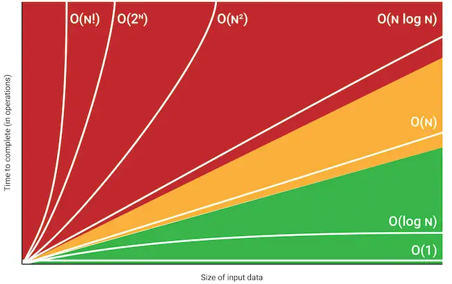
In this article, I will try to give you a brief overview of the different order of complexity of algorithm analysis which is called big O notation. So what is Big O notation is…
- Used to analyze runtime time complexity.
- It provides an abstract measurement by which we can judge the performance of algorithms without using mathematical proofs.
- The entire point of Big-O notation is to be able to compare how efficiently one algorithm solves big problems compared to another.
- One of the great advantages of Big O is that it can give you the complexity of the algorithm without taking into consideration the computing resources, problem size so which makes it a great tool for algorithm analysis.
- Big-O notation is a metric for algorithm scalability.
Most common big Oh notations with examples:
O(1)- Constant complexity:
No matter what you provide as an input to the algorithm, it’ll still run in the same amount of time. The operation doesn’t depend on the size of its input.
1 item, 1 ms
10 items, 1 ms
100 items, 1 ms
Examples:
- Determining if a binary number is even or odd.
- Adding a node to the tail of a linked list where we always maintain a pointer to the tail node.
O(n) - Linear complexity:
The calculation time increases at the same pace as the input. The run time complexity is proportionate to the size of n.
1 item, 1 ms
10 items, 10 ms
100 items, 100 ms
Example:
- Unsorted list search.
O(log n) - Logarithmic complexity:
The calculation time barely increases as you exponentially increase the input numbers, normally associated with algorithms that break the problem into similar chunks per each invocation.
1 item, 1 ms
10 items, 2 sms
100 items, 3 ms
Example: Searching a binary search tree
O(n log n):
This is usually associated with an algorithm that breaks the problem into smaller chunks per each invocation, and then takes the results of these smaller chunks and stitches them back together. It’s like “doing log(n) work n times. For example, searching for an element in a sorted list of length n is O(log n). Searching for the element in n different sorted lists, each of length n is O(n log n).
Example:
- Quicksort
- Merge sort
O(n2) - Quadratic complexity:
The calculation time increases at the pace of n2.
1 item, 1 ms
10 items, 100 ms
100 items, 10,000 ms
Example:
- Bubble sort.
O(n3) - Cubic complexity:
Very rare
O(2n) - Exponential:
Incredibly rare.
O(n!) - Factorial complexity
The calculation time increases at the pace of n!, which means if n is 5, it’s 5x4x3x2x1, or 120. This isn’t so bad at low values of n, but it quickly becomes impossible.
N=1, 1 option
N=10, 3,628,800 options
N=100, 9.332621544×10157 options
Example: Traveling Salesman Problem
Summary and notes:
The biggest asset that big Oh notation gives us is that it allows us to essentially discard things like hardware which means if you have two sorting algorithms, one with a quadric run time and the other with a logarithmic run time then the logarithmic algorithm will always be faster than the quadratic one when the data set becomes suitably large. This applies even if the former is ran on a machine that is far faster than the latter, Why? Because big Oh notation isolates a key factor in algorithm analysis: growth. An algorithm with quadratic run time grows faster than one with a logarithmic run time. It is generally said at some point n->m the logarithmic will become faster than the quadratic algorithm.
Cubic and exponential algorithms should only ever be used for very small problems (if ever!); avoid them if feasibly possible. If you encounter them then this is really a signal for you to review the design of your algorithm always look for algorithm optimization particularly loops and recursive calls.
In my next post, I will try to give an overview of the algorithm complexity of some of the widely used Machine Learning algorithms.
Have great learning!